JUnitBenchmarks:
API & Code Examples
API overview, quick dive
There are two key elements to master: annotations and global system properties. Luckily, most of these are optional and only required if one wants to achieve some specific goal (there are several scenarios discussed below).
Turning your JUnit tests into benchmarks
The assumption is your benchmark is already a JUnit4 test. For example, let's say your test class looks like this:
    public class MyTest {
      @Test
      public void twentyMillis() throws Exception {
        Thread.sleep(20);
      }
    }
To turn it into a benchmark, you must add a JUnit4 rule that tells JUnit runners to attach benchmarking code to your tests. Adding such a rule is easy, just add a field, like so (import statements omitted):
    public class MyTest {
      @Rule
      public MethodRule benchmarkRun = new BenchmarkRule();

      @Test
      public void twentyMillis() throws Exception {
        Thread.sleep(20);
      }
    }
Alternatively, your test class can extend AbstractBenchmark, which declares this field for you:
    public class MyTest extends AbstractBenchmark {
      @Test
      public void twentyMillis() throws Exception {
        Thread.sleep(20);
      }
    }
When you run this test using any JUnit4 runner, it is already a benchmark and the results will be printed to the console. Note the test's execution time in Eclipse, for example:

It is much larger than the sleep interval we set in the sleep method. It is so because benchmarks are repeated multiple times to get a better estimation of the actual average execution time of the tested method. The message printed to the console contains the details for this particular example:
MyTest.twentyMillis: [measured 10 out of 15 rounds]
 round: 0.02 [+- 0.00], round.gc: 0.00 [+- 0.00], GC.calls: 0, GC.time: 0.00,
 time.total: 0.32, time.warmup: 0.12, time.bench: 0.20
The test was therefore repeated 15 times: 5 initial rounds were discarded, for the 10 following rounds the execution time was measured and contributed to the average called round, which is exactly 0.02 seconds or 20 milliseconds. Additional information includes the number of times garbage collector was called and the time spent doing garbage collection. We will interpret these clues later on.
Tuning your benchmarks with annotations
Basic benchmarking above can be tuned to one's needs using additional annotations on test methods. For example, the number of warmup and benchmark rounds can be adjusted with BenchmarkOptions annotation as shown below.
    public class MyTest extends AbstractBenchmark {
      @BenchmarkOptions(benchmarkRounds = 20, warmupRounds = 0)
      @Test
      public void twentyMillis() throws Exception {
        Thread.sleep(20);
      }
    }
We set the number of benchmark passes to 20 and the number of warmup rounds to zero, effectively causing the benchmark to measure all executions of the test method. Next section gradually introduces more of these tuning annotations, showing their use in context.
A full step-by-step benchmarking process
Design your test case and run initial benchmarks
Let's say our task is to compare the performance of three standard Java list implementations: ArrayList, Vector and LinkedList. First of all, we need to design a test case that mimics the code of our eventual application. Let's assume the application adds some elements to the list and then removes elements from the list in random order. The following test does just this:
public class Lists1
{
    private static Object singleton = new Object();
    private static int COUNT = 50000;
    private static int [] rnd;

    /** Prepare random numbers for tests. */
    @BeforeClass
    public static void prepare()
    {
        rnd = new int [COUNT];

        final Random random = new Random();
        for (int i = 0; i < COUNT; i++)
        {
            rnd[i] = Math.abs(random.nextInt());
        }
    }

    @Test
    public void arrayList() throws Exception
    {
        runTest(new ArrayList<Object>());
    }

    @Test
    public void linkedList() throws Exception
    {
        runTest(new LinkedList<Object>());
    }

    @Test
    public void vector() throws Exception
    {
        runTest(new Vector<Object>());
    }

    private void runTest(List<Object> list)
    {
        assert list.isEmpty();

        // First, add a number of objects to the list.
        for (int i = 0; i < COUNT; i++)
            list.add(singleton);

        // Randomly delete objects from the list.
        for (int i = 0; i < rnd.length; i++)
            list.remove(rnd[i] % list.size());
    }
}
Note the following key aspects of the above code:
- the pseudo-random deletion sequence is created once and remains fixed for all tests,
- the test code uses singleton object to avoid allocating memory other than the lists',
- the test is very simple, perhaps overly simple; in real life, you'd like something that resembles your application's use-case scenario.
To turn this test into a micro-benchmark, we will add the familiar BenchmarkRule.
    @Rule
    public MethodRule benchmarkRun = new BenchmarkRule();
When this test is re-run in Eclipse, we will get the following result on the console:
Lists1.arrayList: [measured 10 out of 15 rounds]
 round: 0.60 [+- 0.00], round.gc: 0.00 [+- 0.00], GC.calls: 15, GC.time: 0.02,
 time.total: 9.02, time.warmup: 3.01, time.bench: 6.01
Lists1.linkedList: [measured 10 out of 15 rounds]
 round: 1.14 [+- 0.07], round.gc: 0.00 [+- 0.00], GC.calls: 23, GC.time: 0.07,
 time.total: 17.09, time.warmup: 5.67, time.bench: 11.43
Lists1.vector: [measured 10 out of 15 rounds]
 round: 0.60 [+- 0.01], round.gc: 0.00 [+- 0.00], GC.calls: 15, GC.time: 0.00,
 time.total: 9.04, time.warmup: 3.02, time.bench: 6.02
The difference between the random-access lists (Vector and ArrayList) and a LinkedList is clearly seen in the round time. Another difference is the much longer GC time (and the number of GC calls), resulting from more work the GC must perform on internal node structures in LinkedList (although this is only a wild guess).
There is no observable difference between thread-safe Vector and un-synchronized ArrayList. In fact, the locks inside Vector are uncontended, so the JVM most likely removed them entirely. Now, just by upgrading the JVM to a newer version (from 1.5.0_18 to 1.6.0_18) the results change a lot, compare:
Lists2.arrayList: [measured 10 out of 15 rounds]
 round: 0.25 [+- 0.01], round.gc: 0.00 [+- 0.00], GC.calls: 1, GC.time: 0.00,
 time.total: 3.77, time.warmup: 1.29, time.bench: 2.48
Lists2.linkedList: [measured 10 out of 15 rounds]
 round: 1.27 [+- 0.02], round.gc: 0.00 [+- 0.00], GC.calls: 1, GC.time: 0.00,
 time.total: 19.16, time.warmup: 6.42, time.bench: 12.74
Lists2.vector: [measured 10 out of 15 rounds]
 round: 0.24 [+- 0.00], round.gc: 0.00 [+- 0.00], GC.calls: 0, GC.time: 0.00,
 time.total: 3.73, time.warmup: 1.28, time.bench: 2.45
Random-access lists are almost three times faster than before, while linked-list is even slower than it was, but without (global) GC-activity. Just to stress this again: this is the same code, the same machine, just a different virtual machine in action. Why this is the case, we will leave as an exercise to the reader.
Changing benchmark options
If you wish to alter the default number of rounds or other aspects of the benchmarking environment, use BenchmarkOptions annotation. It can be applied to methods or classes. Benchmarked methods inherit options in the following order:
- global options passed via system properties (if override is enabled),
- method-level BenchmarkOptions annotation,
- class-level BenchmarkOptions annotation,
- framework defaults.
JUnit-benchmarks hints a full GC before every method run to ensure similar test conditions for every invocation. In practice, methods will not be executed with a cleaned heap, so it may be sensible to disable GC-ing of memory and simply take an average from multiple test runs. We thus add the following declaration to the class (it is inherited by all methods):
@BenchmarkOptions(callgc = false, benchmarkRounds = 20, warmupRounds = 3)
We will re-run the benchmarks now, using an even newer JVM (1.7.0, ea-b83). We get:
Lists2.arrayList: [measured 20 out of 23 rounds]
 round: 0.12 [+- 0.00], round.gc: 0.00 [+- 0.00], GC.calls: 0, GC.time: 0.00,
 time.total: 2.76, time.warmup: 0.39, time.bench: 2.36
Lists2.linkedList: [measured 20 out of 23 rounds]
 round: 0.82 [+- 0.01], round.gc: 0.00 [+- 0.00], GC.calls: 1, GC.time: 0.00,
 time.total: 18.78, time.warmup: 2.48, time.bench: 16.30
Lists2.vector: [measured 20 out of 23 rounds]
 round: 0.12 [+- 0.00], round.gc: 0.00 [+- 0.00], GC.calls: 1, GC.time: 0.00,
 time.total: 2.80, time.warmup: 0.40, time.bench: 2.40
Impressive, huh?
Persistent benchmark history
While you work on your code and experiment, it is useful to store the results of each benchmark run in a persistent form, so that results can be compared later on. Or, for that matter, you may wish to set up an automated build that runs benchmarks on different virtual machines, stores the results in the same database and then draws graphical comparison of results. For this, junit-benchmarks provides a persistent storage in a file-based, relational database H2.
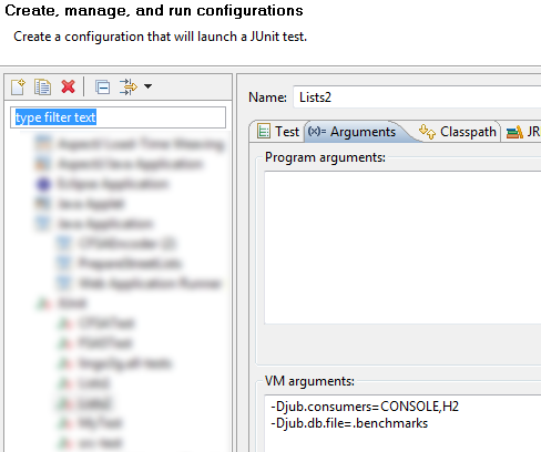
To enable persistent storage, define the following global system properties:
- jub.consumers defines a list of consumers for the results of benchmark runs. By default, this property is set to CONSOLE, but any of the following constants (or a number of them, comma-separated) will do: H2, XML, CONSOLE.
- jub.db.file defines the path to H2 database file in the local filesystem (H2 consumer must be added).
In Eclipse, these properties can be typed into JVM arguments, as in the figure below.
Drawing charts for comparisons
Figures will tell you much, but a picture is worth a thousand digits... or something. Still in Eclipse, let's add the following annotation to the test class:
@AxisRange(min = 0, max = 1)
@BenchmarkMethodChart(filePrefix = "benchmark-lists")
This annotation causes junit-benchmark's H2-based consumer to draw a chart comparing the results of all methods inside the class. Once the JUnit run is finished, a new file will be created in the project's default folder: benchmark-lists.html and benchmark-lists.json. The HTML file is written using Google Charts and requires an internet connection. Once opened, the chart looks like this:

A different type of graphical visualization shows the history of benchmark runs for a given class (and all of its test methods). Let's compare different JVMs using this chart. We will run the same JUnit test from Eclipse using different JVMs each time and adding a custom run key so that we know which run corresponded to which JVM. The custom key is a global system property and is stored in the H2 database together with the run's data. We will set it to the name of each JVM. We execute Eclipse JUnit test four times, each time changing the JRE used for the test and modifying jub.customkey property.
Then, we add the following annotation to the test class:
@BenchmarkHistoryChart(labelWith = LabelType.CUSTOM_KEY, maxRuns = 20)
We tun the test again and open the resulting file.

Interestingly, IBM's virtual machine has a visible difference between Vector and ArrayList.
The target directory for chart generation can be changed by passing a global property (see JavaDoc). Do use and experiment with the H2 database directly for more advanced charting or analysis; H2 is a regular SQL database and provides a convenient access GUI via the browser. Start it from command-line using: java -jar lib/h2*.